Building an AI financial market model - Lesson I

Before you can begin with building your own AI Financial Market Model (machine learned), you have to decide on what software to use.  Since I wrote this article in 2007, many new advances have been made in machine learning. Notably the python module Scikit Learn came out and Hadoop was released into the wild.

I’m not overly skilled in coding and programming – I know enough to get by- I settled on RapidMiner.  RapidMiner is a very simple visual programming platform that let’s you drag and drop “operators” into a design canvas. Each operator has a specific type of task related to ETL, modeling, scoring, and extending the features of RapidMiner.

There is a slight learning curve but, it’s not hard to learn if you follow along with this tutorial!

The AI Financial Market Model

First download RapidMiner Studio and then get your market data (OHLCV prices), merge them together, transform the dates, figure out the trends, and so forth. Originally these tutorials built a simple classification type of model that look to see if your trend was classified as being in an “up-trend” or a “down-trend.” The fallacy was they didn’t not take into account the time series nature of the market data and the resulting model was pretty bad.

For this revised tutorial we’re going to do a few things.

1. Install the Finance and Economics, and Series Extensions
2. Select the S&P500 weekly OHLCV data for a range of 5 years. We’ll visualize the closing prices and auto-generate a trend label (i.e. Up or Down)
3. We’ll add in other market securities (i.e. Gold, Bonds, etc) and see if we can do some feature selection
4. Then we’ll build a forecasting model using some of new H20.ai algorithms included in RapidMiner v7.2

All processes will be shared and included in these tutorials. I welcome your feedback and comments.

The Data

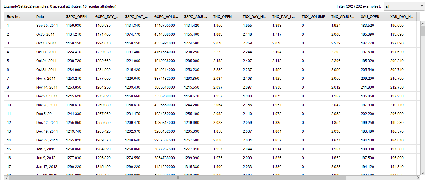
We’re going to use the adjusted closing prices of the S&P500, 10 Year Bond Yield, and the Philadelphia Gold Index from September 30, 2011 through September 20, 2016.

The raw data looks like this:

We renamed the columns (attributes) humanely by removing the “^” character from the stock symbols.

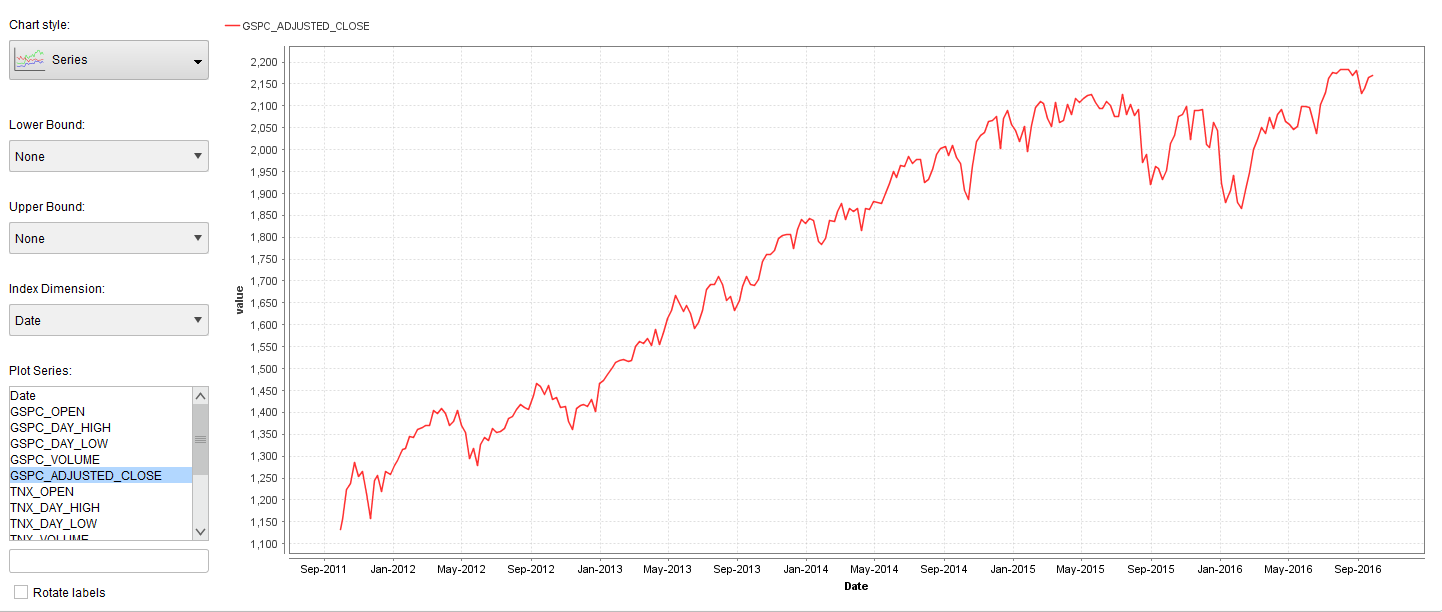
Next we visualized the adjusted weekly closing price of the S&P500 using the built in visualization tools of RapidMiner.

The next step will be to transform the S&P500 adjusted closing price into Up and Down trend labels. To automatically do this we have to install the RapidMiner Series Extension and use the Classify by Trend operator. The Classify by Trend operator can only work if you set the set the SP500_Adjusted_Close column (attribute) as a Label role.

The Label role in RapidMiner is your target variable. In RapidMiner all data columns come in as “Regular” roles and a “Label” role is considered a special role. It’s special in the sense that it’s what you want the machine learned model to learn to. To achieve this you’ll use the Set Role operator. In the sample process I share below I also set the Date to the ID role. The ID role is just like a primary key, it’s useful when looking up records but doesn’t get built into the model.

{{>ga-body}}

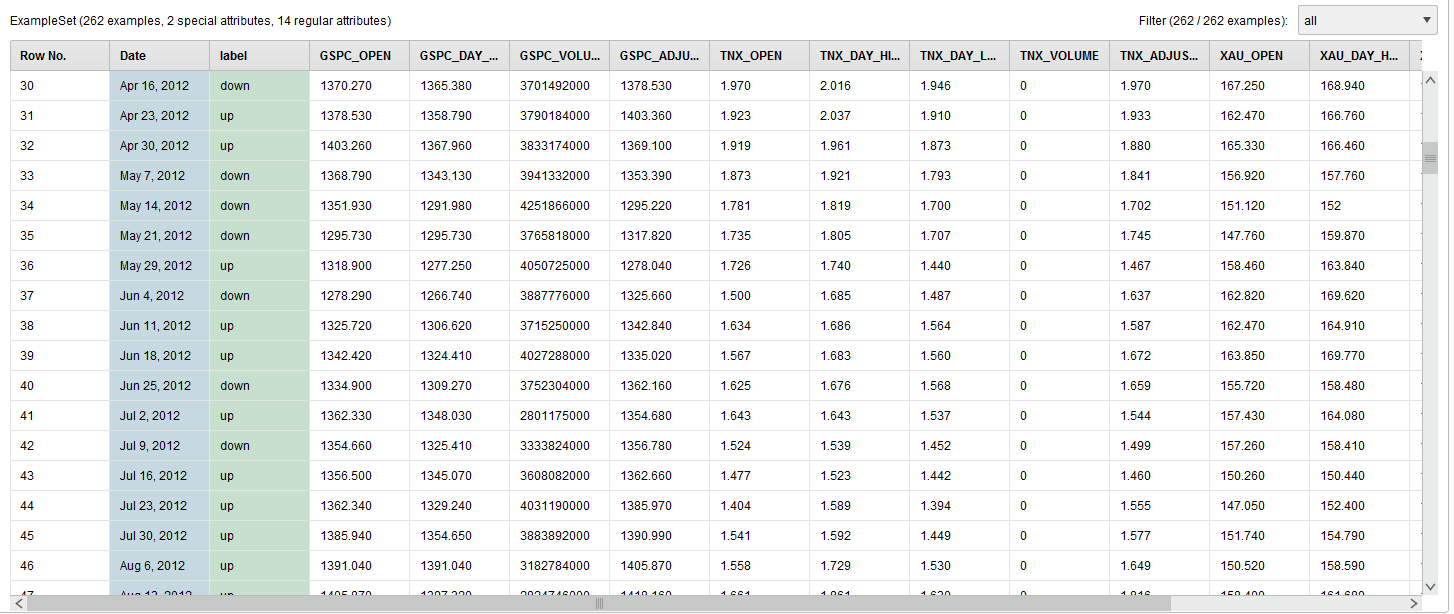
The final data transformation looks like this:

The GSPC_Adjusted_Close column is now transformed and renamed to the label column.

The resulting process looks like this:

That’s the end of Lesson 1 for your first AI financial market model. You can download the above sample process here. To install it, just go to File > Import Process. Lesson 2 will be updated shortly.

_This is an update to my original 2007 YALE tutorials and are updated for RapidMiner v7.0. In the original set of posts I used the term AI when I really meant Machine Learning. _